Home >>STATISTICS, Section 1, regression

Dependent & Independent Variables

Regarding data sets of two variables:

The independent variable (controlled) is the variable representing the value being manipulated/altered.

The dependent variable (outcome) is the observed result.

Example

In an experiment, dependent variables are the factors that are influenced.

So consider an experiment to measure the effect of sunlight on plant growth.

Varying the amount of sunlight is a controlled action.

So this is the independent variable.

The amount of plant growth produced for a given level of light is an outcome.

Therefore plant growth is the dependent variable.

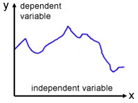
By convention, the dependent variable is on the y-axis, while the independent variable is on the x-axis.

back to top

Scatter Diagrams

The first graph indicates a positive correlation. Points are scattered about a straight line with a positive gradient.

The second graph would have a negative correlation. The line would have a negative gradient.

The third graph would have a correlation close to zero. There is no line in any particular direction indicated.

When two sets of data are plotted against each other, a scatter of points is produced.

Correlation is simply the relationship between one set of data and the other.

It is expressed as a number called the correlation coefficient (r) with values -1 < r < +1 .

back to top

Linear Regression

Regression is a method of describing the relationship between two variables by formulating an equation.

Linear regression is simply where the equation is that of a straight line and has the form:

where 'a' is the intercept on the y-axis and 'b' is the gradient of the line.

The Method of Least Squares

The method relies on the vertical component (y) being the dependent variable and the horizontal component(x) being the independent variable.

This is important when we consider correlation coefficient in detail later.

The formulation of a 'line of best fit' is achieved by examining each point in the scatter.

The vertical distance(e_i) of points above and below the line is recorded and squared.

An equation for the line can be obtained when the sum of the squares given by:

is at a minimum.

When this applies, the gradient b can be expressed in terms of two derived quantities:

S_xy the covariance of x on y

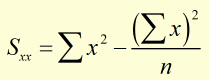
S_xx the variance of x

These are given by:

            (i

               (ii

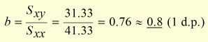
while 'b' , the gradient is given by:

                                                   (iii 

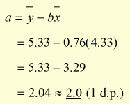
The intercept on the y-axis 'a' is found from:

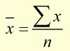
If the mean x and y values are given by:

then,                               

rearranging,

                                  (iv

Method for Solving Problems

Given a list of x-y data, results are found for:

the sum of x  (Σx)

the sum of y (Σy)

the sum of xy (Σxy)

the sum of x² (Σx²)

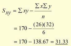
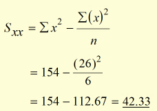
S_xy and S_xx are calculated from equations (i & (ii .

Hence the gradient 'b' is found from (iii .

The mean value of x () is found by dividing Σx by the number of values 'n' .

The mean value of y ()is found by dividing Σy by the number of values 'n' .

Hence the intercept 'a' is found from (iv .

The linear equation is then presented as .

back to top

Example

Given the values of x and y below, find by linear regression an equation representing the data
(gradient & intercept to 1 d.p.).

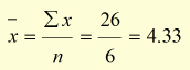
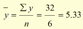
no. data pairs (n) = 6

Using , the equation representing the data is:

back to top

[ About ] [ FAQ ] [ Links ] [ Terms & Conditions ] [ Privacy ] [ Site Map ] [ Contact ]